3 Training Optimisation
The previous chapters established the computational and memory costs of training large models, and the scaling laws that big labs are all chasing. This chapter introduces techniques that make training at scale tractable: mixed-precision training, which reduces memory and increases throughput; gradient accumulation and checkpointing, which enable training with limited GPU memory; Mixture of Experts (MoE), which scales model capacity without proportionally scaling compute; and parameter-efficient fine-tuning methods (LoRA and QLoRA), which adapt large pre-trained models using a fraction of the parameters and memory.
3.1 Gradient Accumulation
The memory requirements computed in Section 1.3 assume standard training where all activations are retained. These activations scale linearly with the batch size, which for stable training can be significant.
Gradient accumulation is a technique that simulates a large batch size using limited GPU memory. Instead of computing the gradient over the full batch in one forward–backward pass, we:
- Perform \(s\) forward–backward passes on micro-batches of size \(b_{\text{micro}}\).
- Accumulate (sum) the gradients across all \(s\) steps.
- Perform a single optimiser update using the accumulated gradient.
The effective batch size is \(b_{\text{eff}} = s \times b_{\text{micro}}\).
Gradient accumulation trades compute time for memory: each micro-batch requires only enough memory for \(b_{\text{micro}}\) samples, but \(s\) sequential forward–backward passes are needed per parameter update. The resulting gradient is mathematically identical to training with batch size \(b_{\text{eff}}\).
In base_train.py, the training loop runs grad_accum_steps forward–backward passes per optimizer step, dividing the loss so that the accumulated gradient has the correct scale:
for micro_step in range(grad_accum_steps):
with autocast_ctx:
loss = model(x, y)
loss = loss / grad_accum_steps
loss.backward()
x, y, _ = next(train_loader)
optimizer.step()
model.zero_grad(set_to_none=True)- 1
- Normalise loss so the accumulated gradient has the correct scale.
- 2
-
Gradients accumulate in
.gradacross micro-steps. - 3
- Single optimiser update on the accumulated gradient, then reset.
3.2 Gradient Checkpointing
Gradient checkpointing (or activation checkpointing) [1] reduces activation memory by selectively discarding intermediate activations during the forward pass and recomputing them during the backward pass.
The key insight is a tradeoff between memory and compute. Consider a model with \(L\) layers. Three strategies span the memory–compute tradeoff:
- Store all activations: Memory \(O(L)\), compute \(O(L)\) (each layer’s forward pass runs once). This is standard training.
- Store no activations: Memory \(O(1)\), compute \(O(L^2)\). Every activation must be recomputed from the input during the backward pass.
- Checkpoint every \(\sqrt{L}\) layers: Memory \(O(\sqrt{L})\), compute \(O(L)\) with a modest constant overhead. Chen et al. showed that this is optimal, reducing memory from \(O(L)\) to \(O(\sqrt{L})\) with at most one extra forward pass per segment. Only \(\sqrt{L}\) activations are stored; during the backward pass, each segment of \(\sqrt{L}\) layers is recomputed from its checkpoint.
Example 3.1 (DeepSeek Gradient Checkpointing) DeepSeek-V3 [2] employs a sophisticated activation compression strategy that goes beyond standard checkpointing. Rather than storing full-precision activations at checkpoint boundaries, they compress the stored activations through quantising (Example 3.2) and project some representations to a lower dimensional space (?def-mla).
3.3 Mixed-Precision Training
Mixed-precision training uses different numerical formats for different parts of the computation, balancing memory savings and speed against numerical stability.
BF16 (BrainFloat16) is a 16-bit floating-point format with 1 sign bit, 8 exponent bits, and 7 fraction bits. It was developed at Google Brain specifically for deep learning and first implemented in Google’s TPU hardware. The design of BF16 reflects a key empirical insight: deep learning models are more sensitive to the range of representable values (determined by the exponent) than to precision (determined by the fraction). By keeping the same 8-bit exponent as FP32, BF16 can represent the same range of magnitudes (\(\sim 10^{-38}\) to \(\sim 10^{38}\)), avoiding the underflow and overflow issues that plague FP16 (which has only a 5-bit exponent).
Mixed-precision training stores the model weights, gradients, and intermediate computations in BF16 (2 bytes each), but maintains a master copy of the weights in FP32 (4 bytes) for the optimiser update. The total memory per parameter is therefore: \[ \underbrace{2P}_{\text{BF16 weights}} + \underbrace{2P}_{\text{BF16 gradients}} + \underbrace{4P}_{\text{FP32 master}} + \underbrace{8P}_{\text{Adam states}} = 16P \;\text{bytes}, \] compared to \(16P\) bytes for pure FP32 training (\(4P\) weights + \(4P\) gradients + \(8P\) Adam). The savings come primarily from activations and communication: intermediate activations are stored in BF16 (halving activation memory), and data transferred between GPUs during distributed training is halved. Note that for small batch sizes, the FP32 master copy can increase total memory, since we store both BF16 and FP32 copies of the weights; the savings become significant only when activation memory dominates.
Example 3.2 (DeepSeek FP8 Training Strategy) DeepSeek-V3 [2] was one of the first large-scale models to successfully use FP8 precision during pre-training, pushing precision even lower than BF16 for the most compute-intensive operations. The FP8 format used is E4M3: 1 sign bit, 4 exponent bits, and 3 mantissa bits. This provides a range of approximately \(\pm 448\) with very coarse precision. E4M3 can represent only \(2^8 = 256\) distinct values, compared to BF16’s \(2^{16} = 65{,}536\).
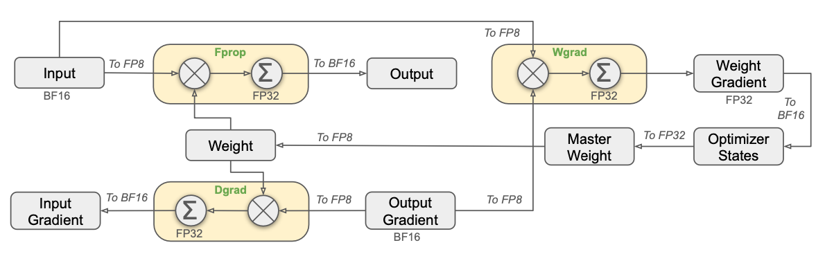
DeepSeek’s approach to making FP8 training work involves several key principles: Selective precision. Not all operations are performed in FP8. Only the high-compute operations—primarily large matrix multiplications (GEMM operations in the MLP and attention layers)—use FP8. Low-compute operations such as layer normalisation, residual additions, softmax, and the router remain in BF16 or FP32. The rationale is straightforward: low-compute operations contribute negligibly to total runtime, so keeping them in higher precision costs almost nothing in speed but avoids introducing quantisation error in numerically sensitive computations. The router, in particular, must remain in high precision because small errors in routing scores can cascade into completely different expert assignments. Fine-grained tile-wise quantisation. Rather than quantising an entire weight matrix with a single scaling factor (which would be sensitive to outliers, as discussed in Section 3.6), DeepSeek divides matrices into small tiles and quantises each tile independently with its own scaling factor. This is the same principle as block-wise quantisation in QLoRA, but applied at the level of matrix tiles during forward computation. Thorough small-scale experimentation. Before committing to FP8 for the full training run, DeepSeek conducted extensive experiments at smaller scales to validate that FP8 training converges to the same loss as BF16 training—a practical application of the scaling laws from Chapter 2. The DeepSeek-V3 precision strategy.
Dynamic quantisation to FP8. The _to_fp8 helper computes a single scalar scale from the tensor’s max absolute value and casts to FP8:
def _to_fp8(x, fp8_dtype):
fp8_max = torch.finfo(fp8_dtype).max
amax = x.float().abs().max()
scale = fp8_max / amax.clamp(min=1e-12)
x_fp8 = (x.float() * scale).clamp(-fp8_max, fp8_max).to(fp8_dtype)
return x_fp8, scale.reciprocal()- 1
- Maximum representable value: 448 for e4m3, 57344 for e5m2.
- 2
-
Maps
[0, amax]→[0, fp8_max]. - 3
-
Returns inverse scale for
_scaled_mm.
Three-GEMM pattern. A custom autograd function quantises both operands on the fly and calls the hardware FP8 matmul for each of the three GEMMs in a linear layer:
class _Float8Matmul(torch.autograd.Function):
@staticmethod
def forward(ctx, input_2d, weight):
input_fp8, input_inv = _to_fp8(input_2d, torch.float8_e4m3fn)
weight_fp8, weight_inv = _to_fp8(weight, torch.float8_e4m3fn)
ctx.save_for_backward(input_fp8, input_inv, weight_fp8, weight_inv)
return torch._scaled_mm(input_fp8, weight_fp8.t(), ...)
@staticmethod
def backward(ctx, grad_output):
in_fp8, in_inv, w_fp8, w_inv = ctx.saved_tensors
go_fp8, go_inv = _to_fp8(grad_output, torch.float8_e5m2)
grad_input = torch._scaled_mm(go_fp8, w_fp8, ...)
grad_weight = torch._scaled_mm(go_fp8.t(), in_fp8, ...)
return grad_input, grad_weight- 1
- Quantise both operands to FP8 e4m3.
- 2
- Save the FP8 tensors (not the original FP32/BF16) for the backward pass — this halves activation memory for these layers.
- 3
- GEMM 1: forward output.
- 4
- Reuse FP8 tensors saved from the forward pass.
- 5
- Quantise gradient to e5m2 (wider dynamic range for gradients).
- 6
-
GEMM 2:
grad_out @ weight. - 7
-
GEMM 3:
grad_out.T @ input.
To enable FP8, every eligible nn.Linear in the model is converted to a Float8Linear that uses _Float8Matmul internally.
3.4 Mixture of Experts
For a standard transformer, roughly two thirds of the parameters in a network reside in the feed-forward (MLP) layers and each MLP matrix is applied independently to each token/representation. Mixture of Experts architectures deviate from this by routing each token to a subset of specialised sub-networks. This results in each token seeing far fewer parameters than than the full model, allowing the total number of parameters to grow much larger than the compute budget would normally allow.
Mixture of Experts (MoE) layer [3] replaces the single feed-forward network in a transformer layer with \(N_e\) parallel expert networks \(\{\mathrm{FFN}_1, \ldots, \mathrm{FFN}_{N_e}\}\) and a router network that determines which experts process each token.
The router is a lightweight network (typically a single linear layer followed by a softmax) that produces a probability distribution over experts for each input token \(\mathbf{x}\):
\[ g_i(\mathbf{x}) = \sigma(\mathbf{x}^\top \mathbf{e}_i), \quad i = 1, \ldots, N_e \tag{3.1}\]
where \(\mathbf{e}_i\) is the learned embedding for expert \(i\). In top-\(K\) gating, only the \(K\) experts with the highest affinity scores are activated:
\[ \mathbf{y} = \sum_{i \in \text{top-}K} g_i(\mathbf{x}) \cdot \mathrm{FFN}_i(\mathbf{x}). \tag{3.2}\]
The output is a weighted combination of only the \(K\) active expert outputs. The affinity scores can be interpreted as a soft routing decision, allowing the model to learn which experts are best suited for different types of inputs. The key advantage of MoE is the decoupling of total parameters from active parameters, allowing much greater model capacity without a proportional increase in compute.
3.4.1 Routing Collapse
A critical challenge in MoE training is ensuring that all experts receive a balanced share of tokens. Routing collapse occurs when the router consistently sends the majority of tokens to a small subset of experts, leaving most experts undertrained. This is a natural failure mode because the router and experts co-adapt: experts that receive more tokens become better, which makes the router send them even more tokens, creating a positive feedback loop. Worse still, an expert that receives no tokens produces no gradients, so it cannot improve and remains permanently neglected. The same applies to the router’s scores for that expert: since it was not selected in the top-\(K\), the router receives no gradient signal suggesting it should start routing tokens there.
Several mitigation strategies have been proposed:
Token dropping. If an expert is overloaded (receives more tokens than a capacity threshold), excess tokens are simply dropped—their FFN computation is skipped. This prevents any single expert from dominating but can harm training quality and threaten overloading nodes if experts are distributed across multiple nodes (more on this later). I am not a fan of this approach!
Auxiliary loss. An additional loss term penalises unbalanced expert utilisation [3]. This is added to the main language modelling loss to encourage the router to distribute tokens more evenly. However, tuning the auxiliary loss coefficient is delicate: too strong and it interferes with the primary objective; too weak and it fails to prevent collapse.
Example 3.3 (DeepSeek-V3 MoE Configuration) 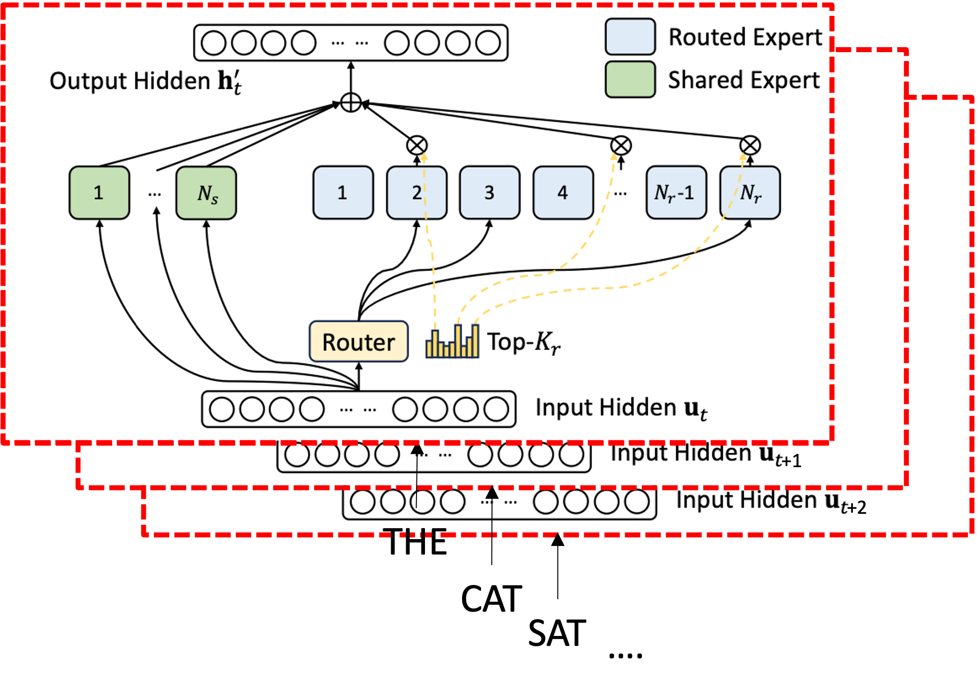 DeepSeek-V3 [2] adapted the standard MoE architecture with \(N_e = 256\) routed experts, significantly more than what was seen previously (Mistral models tended to have \(N_e = 8\)), and introduced the concept of a shared expert. Each token activates the top-\(K = 8\) of 256 experts, giving a total of 671B parameters but only $$37B activated per token.
Node-limited routing. Experts are often distributed across multiple GPU nodes, each hosting a subset of experts. When a token is routed to an expert on a different node, it must be sent across the inter-node network, making communication a key bottleneck. To address this, DeepSeek-V3 constrains each token to be sent to at most \(M = 4\) compute nodes, where the top \(K/M = 2\) experts per node are selected by the sum of their affinity scores. This reduces inter-node communication overhead by constraining the communication pattern while preserving expert diversity.
Bias adjustment for expert load balancing/avoiding routing collapse. Rather than using an auxiliary loss, DeepSeek-V3 directly adjusts the router by adding or subtracting a bias term to the affinity scores. The bias is adjusted dynamically: an overloaded expert has its bias decreased; an underutilised expert has its bias increased. This avoids the need for a carefully tuned auxiliary loss coefficient.
nanochat’s moe.py (on the moe branch) implements a DeepSeekV3-style MoE as a drop-in replacement for the dense MLP.
Router. A sigmoid-gated top-\(K\) router scores every expert and picks the best \(K\). Bias-based load balancing nudges underused experts up and overloaded experts down — no auxiliary loss needed:
scores = torch.sigmoid(self.gate(x).float())
biased_scores = scores + self.expert_bias
_, selected_experts = torch.topk(biased_scores, k=self.top_k, dim=-1)
top_scores = scores.gather(dim=-1, index=selected_experts)
mean_count = counts.mean()
self.expert_bias += coeff * torch.sign(mean_count - counts)- 1
- Bias affects selection only, not the final gating weights.
- 2
- Gather the unbiased scores for the selected experts.
- 3
- Bias update: nudge toward uniform load — overloaded experts decrease, underused experts increase.
Expert dispatch. Tokens are sorted by expert assignment so each expert’s tokens are contiguous, then all experts run in one kernel via torch._grouped_mm:
token_indices_sorted = torch.argsort(selected_experts.view(-1), stable=True)
routed_input = x_flat[token_ids] * scores_sorted.unsqueeze(-1)
offsets = torch.cumsum(num_tokens_per_expert, dim=0, dtype=torch.int32)
h = torch._grouped_mm(x_bf16, w_up_bf16, offs=offsets)
h = F.relu(h).square()
routed_output = torch._grouped_mm(h.bfloat16(), w_down_bf16, offs=offsets)- 1
- Pre-weight tokens by their router scores.
- 2
- Offsets mark where each expert’s tokens begin in the sorted array.
- 3
-
_grouped_mmruns all expert matmuls in a single kernel. - 4
- Squared ReLU activation.
Shared expert. A standard dense MLP that runs on all tokens alongside the routed path — launched before routed experts so compute can overlap:
shared_output = self.shared_expert(x_flat)
output = routed_output + shared_output- 1
- Combine routed and shared paths.
3.5 LoRA: Low-Rank Adaptation
After pretraining we may want to adapt our model to a specific downstream task. The pretrained weights \(\Phi\) are updated \(\Phi + \Delta\Phi\) according to
\[ \max_{\Phi} \sum_{(x,y) \sim \mathcal{Z}} \sum_{t=1}^{|y|} \log P_{\Phi}(y_t \mid x, y_{<t}) \]
where \(\mathcal{Z}\) is the fine-tuning dataset and \(x\), \(y\) are the context and target tokens respectively. Here, every parameter in \(\Phi\) is updated, therefore we need to store gradients and optimiser states for every weight. If we want a bespoke model for each downstream task, a new model of size \(|\Phi|\) is required, and we need to relearn \(|\Delta\Phi|\) parameters. As we know from Section 1.3, this is prohibitively expensive for large models.
Although neural network loss landscapes are often described as highly non-convex and tricky to traverse, Goodfellow et al. [4] observed that the 1-D slice of the loss along the interpolation from initial parameters \(\theta_i\) to the final optimised parameters \(\theta_f\) is often simple, never meets obstacles and is roughly convex — i.e., evaluating \(J((1-\alpha)\theta_i + \alpha\theta_f)\) for \(\alpha \in [0,1]\) yields a nearly convex curve. This suggests that if we knew the direction to take at the start of training, a simple straight path through parameter space would yield good results.
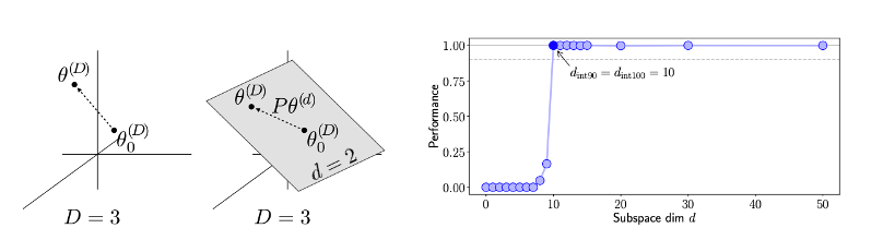
LoRA provides an elegant alternative based on observations that the weight updates during fine-tuning have low intrinsic dimensionality. The theoretical motivation comes from work on the structure of neural network loss landscapes. Li et al. [5] showed that, for many neural networks, the loss can be optimised almost as well within a much lower-dimensional subspace than the full parameter space by training only in a random linear subspace of the specified dimensionality (i.e., projecting gradients onto a fixed random basis). This can be seen in Figure 3.2 where at a subspace dim of 10 the performance is already saturated. Aghajanyan et al. [6] extended this observation to language model fine-tuning, finding that the intrinsic dimensionality of the fine-tuning objective tends to decrease as models grow larger.
LoRA freezes the pre-trained weight matrix \(W_0 \in \R^{d \times k}\) and adds a trainable low-rank decomposition.
The output of a LoRA-adapted linear layer is
\[ \mathbf{h} = W_0 \mathbf{x} + \frac{\alpha}{r} L_2 L_1 \mathbf{x}, \tag{3.3}\]
where \(L_2 \in \R^{d \times r}\) and \(L_1 \in \R^{r \times k}\) with rank \(r \ll \min(d, k)\). Only \(L_1\) and \(L_2\) are trained; \(W_0\) remains frozen. The scalar \(\alpha / r\) controls the magnitude of the low-rank update relative to \(W_0\). Crucially, \(L_2\) is initialised to zero (and \(L_1\) to a random Gaussian) so that \(\Delta W = L_2 L_1 = 0\) at the start of training, this preserves the pre-trained model’s behaviour at step 0 and ensures stable training.
The number of trainable parameters per adapted layer is \(r(d + k)\), compared to \(dk\) for full fine-tuning, a reduction by a factor of approximately \(dk / r(d+k) \approx d / 2r\) when \(d = k\). For a weight matrix of size \(d \times d = 4096 \times 4096\) with LoRA rank \(r = 8\):
\[ \begin{aligned} \text{Full fine-tuning:} &\quad 4096^2 = 16{,}777{,}216 \text{ parameters} \\ \text{LoRA:} &\quad 8 \times (4096 + 4096) = 65{,}536 \text{ parameters} \end{aligned} \]
This is a \(256\times\) reduction.
Example 3.4 (LoRA Memory Savings for LLaMA-65B) How much GPU memory does this save? With LoRA rank 16 on all linear layers, LLaMA-65B has approximately 200M trainable parameters (4 attention projections + 3 MLP projections per layer × 80 layers), roughly 0.3% of the total. We no longer need gradients or optimiser states for the frozen base model. Comparing with full fine-tuning from Example 1.3:
\[ \begin{aligned} & & \text{Full FT} & & \text{LoRA} \\ \hline \text{Weights (FP32):} & & 260 \;\text{GB} & & 260 \;\text{GB} \\ \text{LoRA parameters (BF16):} & & - & & 0.4 \;\text{GB} \\ \text{Gradients:} & & 260 \;\text{GB} & & 0.4 \;\text{GB} \\ \text{Adam states:} & & 520 \;\text{GB} & & 1.6 \;\text{GB} \\ \text{Activations (batch 1):} & & 250 \;\text{GB} & & 250 \;\text{GB} \\ \hline \text{Total:} & & 1{,}290 \;\text{GB} & & \approx 512 \;\text{GB} \end{aligned} \]
LoRA has several nice properties. At inference time, the LoRA matrices can be merged: \(W = W_0 + L_2 L_1\). The resulting model has exactly the same architecture and computational cost as the original. This also enables adapter swapping, where different LoRA adapters (for different tasks or users) can be dynamically loaded and merged with the same base model.
Hu et al. showed that LoRA with rank \(r = 1\) is often competitive with higher ranks, suggesting that the fine-tuning updates are extremely low-rank. This is a striking result: a single rank-1 update per layer, adding just \(d + k\) parameters, can meaningfully adapt a model with billions of parameters. In practice, ranks of \(r = 4\) to \(r = 16\) are most commonly used.
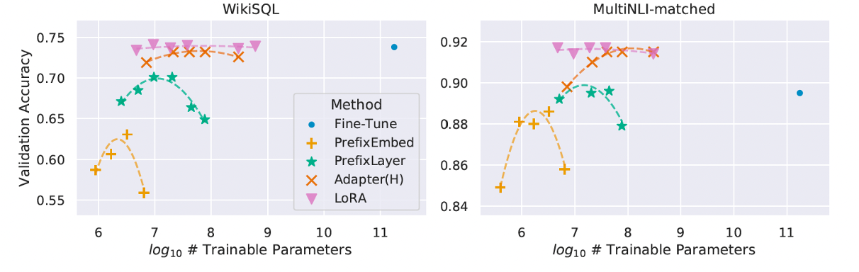
Example 3.5 (Where to Place Adapters and Why Small Ranks Work for GRPO/RL) Recent large-scale experiments by Schulman et al. (Thinking Machines) investigate when it is best to apply LoRA or full fine-tuning in post-training regimes [8]. Their headline result is that LoRA can match full finetuning in both learning speed and final performance for typical instruction-tuning and reasoning datasets, provided two conditions hold: (i) LoRA is applied broadly across the network (not only attention layers as suggested in [7]), and (ii) the adapter is not capacity-constrained by the amount of information in the training signal.
The information-capacity perspective is an interesting one: LoRA behaves like full finetuning until it runs out of capacity, at which point learning becomes less efficient and falls off the best achievable training curve (rather than simply hitting a sharp loss floor). In supervised fine-tuning, each example supplies dense token-level supervision, so the effective information content scales roughly with the number of tokens; larger SFT datasets can therefore require higher-rank adapters to avoid becoming capacity-limited. In contrast, for policy-gradient reinforcement learning (including GRPO-like variants [9]), the learning signal per episode is driven primarily by a scalar advantage/reward, so the “information bandwidth” is far lower, on the order of \(O(1)\) bits per episode in an information-theoretic upper-bound sense. This makes it plausible that very small ranks (even \(r = 1\)) can match full finetuning for RL: the adapter simply needs enough parameters to absorb the comparatively small amount of task information conveyed through rewards. Schulman et al. validate this empirically on mathematical reasoning RL, finding LoRA and full finetuning reach essentially the same peak performance across learning-rate sweeps even at tiny ranks. This provides a clean explanation for why LoRA can be especially effective for GRPO-style reasoning RL: the reward channel is information-thin relative to SFT, so adapter capacity requirements are correspondingly modest.
nanochat does not implement LoRA natively — its chat_sft.py does full fine-tuning. Below is what LoRA would look like if added to nanochat’s SFT stage. A wrapper module replaces every nn.Linear, implementing Equation 3.3 in its forward:
class LoRALinear(nn.Module):
def __init__(self, base, r, alpha):
super().__init__()
self.base = base
self.lora_l1 = nn.Linear(base.in_features, r, bias=False)
self.lora_l2 = nn.Linear(r, base.out_features, bias=False)
self.scale = alpha / r
def forward(self, x):
return self.base(x) + self.scale * self.lora_l2(self.lora_l1(x))- 1
- Frozen original layer.
- 2
- Low-rank matrices \(L_1 \in \mathbb{R}^{r \times k}\) and \(L_2 \in \mathbb{R}^{d \times r}\).
- 3
- Scaling factor \(\alpha / r\).
- 4
- Implements Equation 3.3: base output plus scaled low-rank update.
Every nn.Linear in the model is swapped for a LoRALinear, then base parameters are frozen:
for name, module in model.named_modules():
for attr, child in module.named_children():
if isinstance(child, nn.Linear):
setattr(module, attr, LoRALinear(child, r=8, alpha=16))
for name, param in model.named_parameters():
param.requires_grad = 'lora_' in name- 1
-
Replace every
nn.Linearwith aLoRALinearwrapper. - 2
- Freeze all parameters except LoRA matrices.
3.6 QLoRA: Quantised Low-Rank Adaptation
QLoRA [10] extends LoRA by quantising the frozen base model weights to 4-bit precision, dramatically reducing memory requirements (these frozen weights take up 260GB; see Example 3.4). The key insight is that the base weights \(W_0\) are never updated during LoRA fine-tuning, so they can be stored at very low precision.
But 4 bits means only 16 distinct values. How can we represent a weight matrix with so few levels and not destroy model training? Naïve quantisation would be far too lossy. QLoRA makes this work through three innovations: block-wise quantisation to handle outliers, double quantisation to reduce overhead, and NormalFloat4 to optimally place the 16 quantisation levels for neural network weights.
The starting point is absmax quantisation, which maps a floating-point tensor \(\mathbf{x}\) into \(2^b\) evenly spaced levels symmetric around zero by normalising by the maximum absolute value:
\[ \mathbf{x}^{\text{q}} = \left\lfloor \frac{2^{b-1} - 1}{\max |\mathbf{x}|} \cdot \mathbf{x} \right\rceil \tag{3.4}\]
where \(\lfloor \cdot \rceil\) denotes rounding to the nearest level, \(b\) is the number of bits, and the factor \(2^{b-1} - 1\) reflects the symmetric signed range \([-2^{b-1}+1, \; 2^{b-1}-1]\). Dequantisation recovers an approximation by rescaling: \(\hat{\mathbf{x}} = \frac{\max |\mathbf{x}|}{2^{b-1} - 1} \cdot \mathbf{x}^{\text{q}}\).
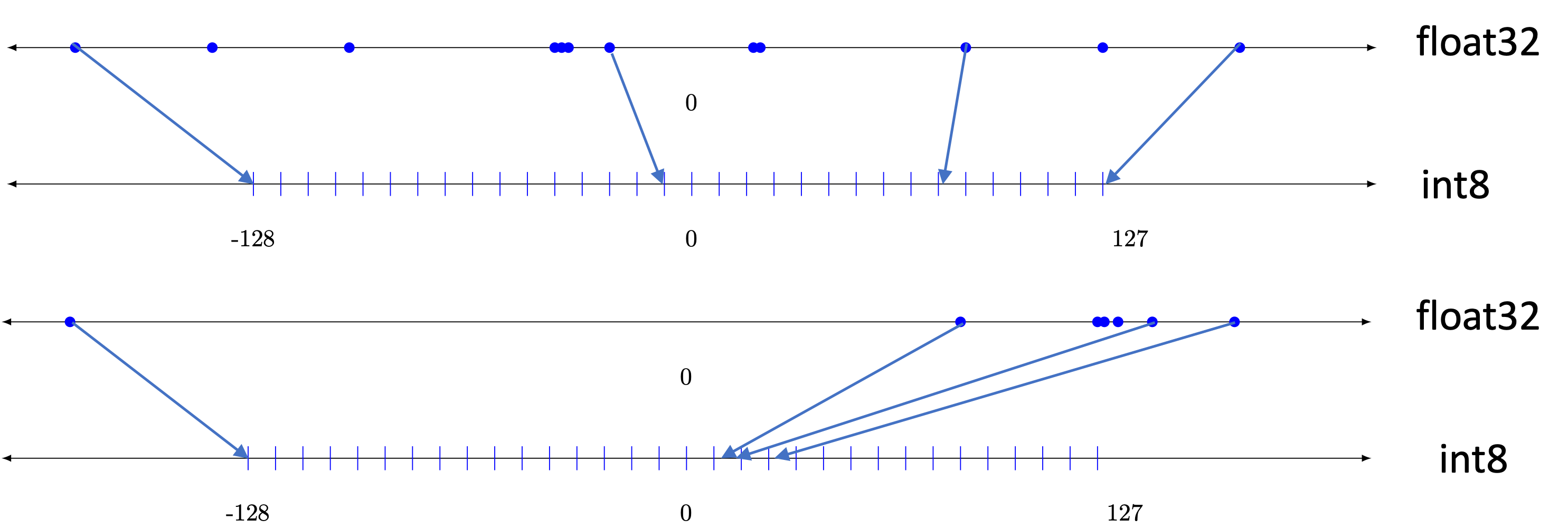
The immediate problem is outliers: a single extreme value inflates \(\max|\mathbf{x}|\), spreading the 16 available bins across a much wider range than necessary (Figure 3.4). Most weights cluster near zero, so the majority of bins end up assigned to regions where almost no values lie.
Block-wise quantisation mitigates the outlier problem by dividing the weight tensor into contiguous blocks of \(B\) elements (typically \(B = 64\)) and quantising each block independently with its own absmax scaling factor, stored in higher precision. An outlier in one block only affects that block’s bin placement, leaving the remaining blocks unharmed.
Block-wise quantisation introduces overhead: each block of 64 values requires its own FP32 scaling constant, adding 0.5 bits per parameter. Double quantisation reduces this overhead by quantising the scaling constants themselves. The FP32 constants from each group of blocks are gathered (e.g., 256 constants together) and quantised to FP8 with a single FP32 second-level constant. This reduces the per-parameter overhead from 0.5 bits to approximately 0.127 bits.
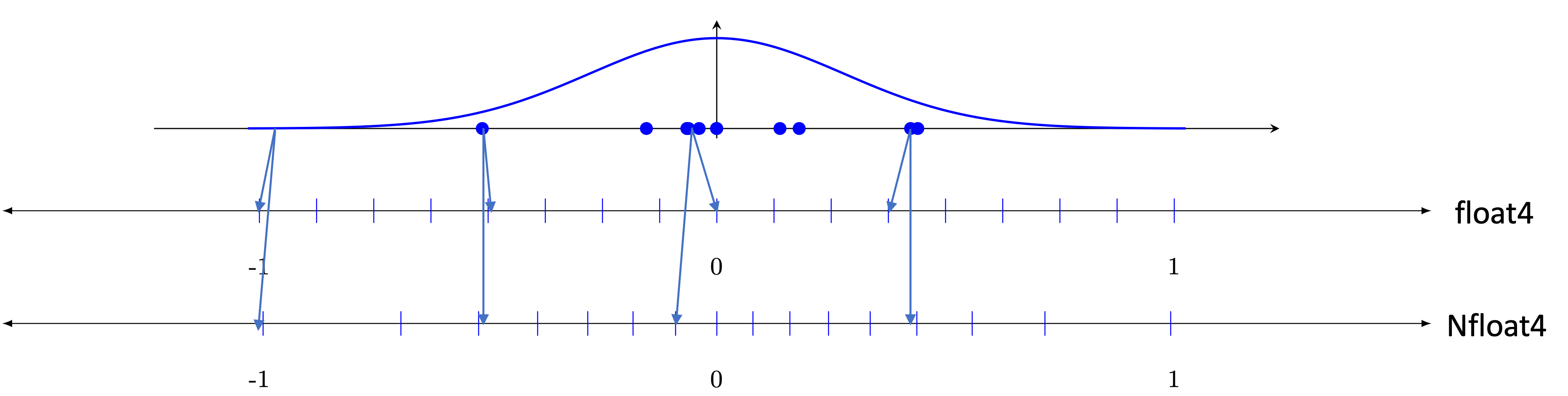
To further reduce information loss (empirically improving performance), QLoRA exploits the fact that pre-trained neural network weights are approximately normally distributed (Figure 3.5). The NormalFloat4 (NF4) data type places its 16 quantisation levels at the quantiles of the standard normal distribution, ensuring equal probability mass in each bin. Because each bin is equally likely to be occupied, no quantisation level is wasted. NF4 is information-theoretically optimal for normally distributed data: it minimises the expected quantisation error among all possible 4-bit codes. The 16 NF4 levels are:
\[ \begin{aligned} &-1.0,\; -0.6962,\; -0.5251,\; -0.3949,\; -0.2844,\; -0.1848,\; -0.0911,\; 0.0, \\ &\phantom{-}0.0796,\; \phantom{-}0.1609,\; \phantom{-}0.2461,\; \phantom{-}0.3379,\; \phantom{-}0.4407,\; \phantom{-}0.5626,\; \phantom{-}0.7230,\; \phantom{-}1.0 \end{aligned} \]
Note the levels are denser near zero, where the normal distribution has most of its mass. The value \(0.0\) is artificially included (replacing the true quantile at that position) because exact zero is a common value in neural networks and must be representable without error.
Dequantisation. The frozen weights are stored in NF4, but computation still requires higher precision. During the forward pass, NF4 weights are dequantised on-the-fly to BF16 for each matrix multiplication: the stored 4-bit index is mapped to its corresponding NF4 quantile value, which is then rescaled by the block’s (doubly-dequantised) scaling factor. The LoRA matrices \(L_1\) and \(L_2\) are kept in BF16 throughout and receive gradients normally. This means the quantisation error is present only in the forward computation through \(W_0\), the gradient updates to the LoRA parameters are exact.
The Triton kernel below implements the three core steps of NF4 block-wise quantisation on the GPU.
Per-block absmax. Each program instance loads a tile of contiguous blocks, reshapes them into a 2D grid of (blocks, BLOCK_SIZE), and computes the maximum absolute value along each row. This per-block scale factor is what makes block-wise quantisation robust to outliers, an extreme value in one block cannot distort the quantisation of any other block:
@triton.jit
def quantize_nf4_blockwise_kernel(
A_ptr, absmax_ptr, out_ptr, n_elements,
BLOCK_SIZE: tl.constexpr, SPLIT_NUM_BLOCKS: tl.constexpr,
):
# ... load a tile of PAIRED_SPLIT_NUM_BLOCKS * BLOCK_SIZE elements ...
A_reshaped = tl.reshape(A, (PAIRED_SPLIT_NUM_BLOCKS, BLOCK_SIZE))
absmax = tl.max(tl.abs(A_reshaped), axis=1)
A_normalized = A_reshaped / absmax[:, None]
A_normalized = tl.clamp(A_normalized, -1.0, 1.0)- 1
-
Reshape flat tile into
(num_blocks, BLOCK_SIZE)so each row is one quantisation block. - 2
- Per-block absmax: reduce along the block dimension. One scale factor per block, stored in higher precision.
- 3
-
Normalise each block into \([-1, 1]\) by dividing by its own absmax.
[:, None]broadcasts the scalar across the block.
Nearest-neighbour quantisation. With values normalised to \([-1, 1]\), the kernel maps each value to one of 16 NF4 codes. Rather than computing distances to all 16 levels, it uses a hard-coded binary decision tree of 15 thresholds — each threshold is the midpoint between two adjacent NF4 levels:
result = tl.where(
A_normalized > 0.03979,
tl.where(
A_normalized > 0.38931,
tl.where(
A_normalized > 0.64279,
tl.where(A_normalized > 0.86148, 0b1111, 0b1110),
tl.where(A_normalized > 0.50166, 0b1101, 0b1100),
),
# ... 12 more branches ...
),
# ... negative side (same structure) ...
)
quantized = result.to(tl.uint8)- 1
- First split: positive vs. negative side of the NF4 codebook.
- 2
-
Each leaf assigns a 4-bit code (
0b0000–0b1111). Four levels of nesting = \(\log_2 16\) comparisons per value. - 3
- Each element now holds a code 0–15.
Nibble packing. Each 4-bit code occupies a full uint8 at this point, wasting half the bits. The kernel packs two codes into a single byte, halving the output size:
quantized = quantized.reshape(
(PAIRED_SPLIT_NUM_BLOCKS, BLOCK_SIZE // 2, 2))
left, right = quantized.split()
packed = left << 4 | (right & 0xF)- 1
- Group consecutive pairs of codes along the last axis.
- 2
- Split into the first and second element of each pair.
- 3
- Pack: high nibble = first code, low nibble = second code. One byte now stores two quantised weights, achieving the 0.5 bytes/parameter that makes the memory savings in Example 3.6 possible.
Example 3.6 (QLoRA: Fine-tuning LLaMA-65B on a Single GPU) With QLoRA, the approximate memory footprint for fine-tuning LLaMA-65B becomes (assuming LoRA rank 16 on all linear layers, batch size 1, and gradient checkpointing; compare with the 1,290 GB required for full-precision training from Example 1.3) \(\sim\) 45 GB, fitting within a single 48 GB NVIDIA RTX 6000 or A6000 GPU. This enables fine-tuning a 65B-parameter model—previously requiring a cluster of 25 GPUs—on consumer-grade hardware.
Paged Optimisers
Even at 45 GB, training can hit occasional out-of-memory errors when a long sequence in a mini-batch causes a spike in activation memory. QLoRA addresses this with paged optimisers, which use NVIDIA unified memory to automatically evict optimiser states from GPU to CPU RAM when memory runs low, and page them back in during the optimiser update step. In the common case there is no overhead; only during rare memory spikes does the system spill to CPU rather than crashing. Combined with gradient checkpointing (Section 3.2), which trades recomputation for activation memory, QLoRA makes it practical to fine-tune large models on a single consumer GPU even with variable-length input sequences.