4 Inference Optimisation
The previous chapters focused on reducing the cost of training. This chapter turns to techniques that improve efficiency at inference time: key–value caching, which eliminates redundant computation during autoregressive generation, Multi-Head Latent Attention, which compresses cached representations to reduce memory, and speculative decoding, which generates multiple tokens per forward pass. This is super important for serving large models and rolling out long reasoning traces to maximise performance (see Section 2.2) and generating trajectories for RL training.
4.1 KV Caching
Autoregressive language models generate text one token at a time. A naive implementation recomputes the full attention over all previous tokens at each generation step, leading to massive redundant computation. The key–value (KV) cache stores the key and value projections for all previously generated tokens, so that at each new generation step only the key and value for the new token need to be computed. The insight comes from the causal attention mask: when generating token \(t\), the attention scores for tokens \(1, \ldots, t-1\) do not depend on this new token, so caching avoids recomputing them.
To see why we cache keys and values but not queries, note that during autoregressive decoding at step \(t\) we only need \(\mathbf{o}_t\), the outputs \(\mathbf{o}_1, \ldots, \mathbf{o}_{t-1}\) were already computed and consumed in previous steps. The causal attention output at position \(t\) is: \[ \mathbf{o}_t = \operatorname{softmax}\!\bigl(\mathbf{q}_t^\top [\mathbf{k}_1, \ldots, \mathbf{k}_t]\bigr)\, [\mathbf{v}_1, \ldots, \mathbf{v}_t]^\top. \] This depends on \(\mathbf{q}_t\) (the query for the current token), plus all keys \(\mathbf{k}_1, \ldots, \mathbf{k}_t\) and values \(\mathbf{v}_1, \ldots, \mathbf{v}_t\). The previous queries \(\mathbf{q}_1, \ldots, \mathbf{q}_{t-1}\) are absent: the causal mask means the output at position \(t\) never involves queries from other positions. Conversely, \(\mathbf{k}_j\) and \(\mathbf{v}_j\) for \(j < t\) appear in \(\mathbf{o}_t\) with exactly the same values as when they were first computed, so caching them avoids redundant recomputation. In short: each query is used once (at the step it is generated) and can be discarded, while each key–value pair is reused at every subsequent step and must be retained.
For a model with \(L\) layers, batch size \(b\), sequence length \(n\), key–value head dimension \(d_{\mathrm{kv}}\), number of KV heads \(n_{\mathrm{kv}}\), stored at \(B\) bits per element, the KV cache requires
\[ M_{\text{KV}} = 2 \cdot L \cdot b \cdot n \cdot n_{\mathrm{kv}} \cdot d_{\mathrm{kv}} \cdot \frac{B}{8} \quad \text{bytes}. \tag{4.1}\]
The factor of 2 accounts for both key and value tensors.
Example 4.1 (KV Cache Exceeding Model Size) For a large model serving many concurrent requests with long contexts, the KV cache can exceed the size of the model weights themselves (the model weights are shared across all requests, but each request maintains its own KV cache). For example, consider a model with \(L=80\) layers, \(n_{\mathrm{kv}}=8\) KV heads of dimension \(d_{\mathrm{kv}}=128\), serving \(b=32\) concurrent requests with context length \(n = 32{,}768\) in BF16: \[ M_{\text{KV}} = 2 \times 80 \times 32 \times 32{,}768 \times 8 \times 128 \times 2 \approx 344 \;\text{GB}. \]
The KV cache can also be shared across requests. When multiple requests share the same prefix, such as a system prompt or a shared conversation history, the KV cache for that prefix can be computed once and reused, avoiding redundant prefill. This is particularly valuable in agentic workflows, where each tool-use step appends to the same conversation and would otherwise re-prefill the entire context from scratch.
microGPT is not an efficient transformer implementation, it is an exercise in implementing one in as few lines of Python as possible. In gpt/gpt.py, the cache is just a pair of Python lists, one per layer, that grow as tokens are generated. The gpt() function takes these lists as arguments and appends each new token’s key and value:
def gpt(token_id, pos_id, keys, values):
x = [t + p for t, p in zip(wte[token_id], wpe[pos_id])]
x = rmsnorm(x)
for li in range(n_layer):
q = linear(x, state_dict[f"layer{li}.attn_wq"])
k = linear(x, state_dict[f"layer{li}.attn_wk"])
v = linear(x, state_dict[f"layer{li}.attn_wv"])
keys[li].append(k)
values[li].append(v)
for h in range(n_head):
k_h = [ki[hs:hs+head_dim] for ki in keys[li]]
v_h = [vi[hs:hs+head_dim] for vi in values[li]]
attn_logits = [sum(q_h[j] * k_h[t][j] ...) for t in range(len(k_h))]
...- 1
- Sum token and position embeddings to form the input representation.
- 2
- Project into query, key, and value for the current token only.
- 3
- Append the new key and value to this layer’s cache.
- 4
- Attention reads from all cached keys and values (positions \(0 \ldots \texttt{pos\_id}\)).
At inference time the cache is initialised empty and accumulates across generation steps — each call to gpt() computes only the new token’s key and value, while reading all previously cached ones:
keys, values = [[] for _ in range(n_layer)], [[] for _ in range(n_layer)]
token_id = BOS
for pos_id in range(block_size):
logits = gpt(token_id, pos_id, keys, values)
token_id = sample(logits)- 1
- One empty list per layer — the cache starts with no stored keys or values.
- 2
- Each call appends one key–value pair per layer; the cache grows by 1 at every step.
Prefill–Decode Disaggregation
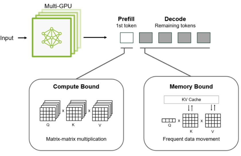
The inference process can be usefully decomposed into two phases with different computational characteristics and optimisation pressures:
Prefill (context processing): A forward pass over the full input context to build attention state (e.g., key–value caches) for each token and layer. Tokens in the prompt are processed in parallel. Prefill latency is a major driver of time to first token (TTFT), the delay before any output is produced. Prefill is often compute-bound (dominated by dense matrix multiplications), though for very long contexts it can become memory/attention-bandwidth sensitive due to attention and cache traffic.
Decode (token generation): Sequential generation of output tokens, happening after the initial prefill stage, typically one token per forward pass. Only the new token’s key and value are computed and appended to the cache, but each step still executes large portions of the model. For large models at small batch sizes, decode is often memory-bandwidth-bound, because the arithmetic per byte of weight traffic is low relative to prefill (weights must be read frequently across many small steps). For long contexts, decode can also become bottlenecked by KV-cache reads (attention over an increasing cache), not only weight reads. Decode performance primarily determines token throughput (tokens/sec), i.e., how fast the response streams after the first token.
These phases have different, often conflicting, optimisation requirements, so when both share the same GPUs they cannot be independently tuned, and scheduling interference can increase tail latency (e.g., heavy prefill work delaying ongoing decode).
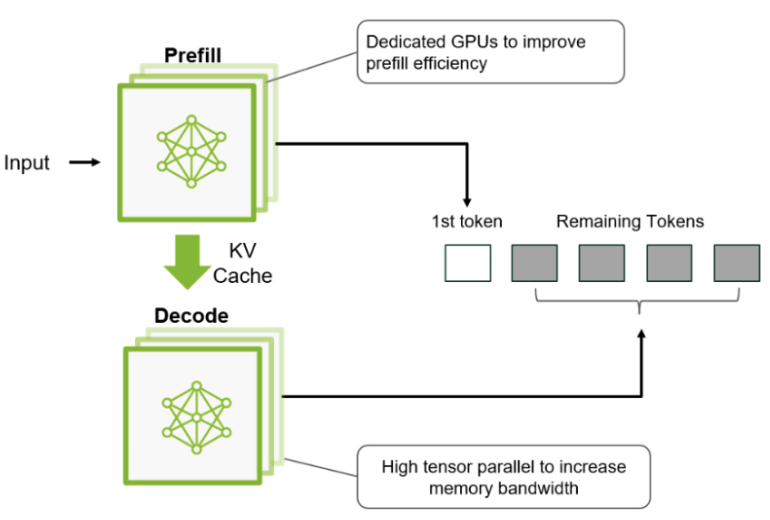
Disaggregation addresses this by separating the phases onto dedicated resources: prefill servers tuned for context throughput/compute efficiency, and decode servers tuned for steady-state generation throughput/bandwidth. This separation can also mitigate queueing interference between prefill and decode workloads. In practice, disaggregation introduces a state-transfer boundary (e.g., moving KV-cache state from prefill to decode servers), which must be engineered carefully so the transfer overhead does not erase the latency/throughput gains.
Example 4.2 (NVIDIA Dynamo) NVIDIA Dynamo is an open-source inference serving framework that implements prefill–decode disaggregation. It routes prefill and decode to separate GPU pools, applies different parallelism strategies to each phase, and manages KV cache transfer between them. Dynamo also supports KV cache offloading to CPU DRAM or SSD: when GPU memory is insufficient, cached keys and values are paged to host memory and fetched back on demand, trading latency for the ability to serve longer contexts or more concurrent requests. Serving DeepSeek-R1 on GB200 NVL72 hardware, Dynamo achieved a 30\(\times\) throughput increase over co-located serving.
4.2 Multi-Head Latent Attention
Even with KV caching, the cache size grows linearly with sequence length and can become a bottleneck for long-context models. Multi-Head Latent Attention (MLA) addresses this by compressing the cached representations.
MLA [1] compresses the key–value representations before caching by projecting them into a low-dimensional latent space via learned projection matrices. Instead of caching the full key and value vectors, MLA caches a compressed latent representation and reconstructs the keys and values on-the-fly during attention computation. For each token \(t\):
Down-project the hidden state \(\mathbf{h}_t \in \R^d\) into a compressed KV latent \(\mathbf{c}_t^{\mathrm{KV}} \in \R^{d_c}\) where \(d_c \ll d\): \[ \mathbf{c}_t^{\mathrm{KV}} = W^{DKV}\, \mathbf{h}_t. \tag{4.2}\]
Cache only \(\mathbf{c}_t^{\mathrm{KV}}\) (dimension \(d_c\)) instead of separate key and value vectors (dimension \(2 \cdot n_h \cdot d_{\text{head}}\)).
Up-project at attention time to reconstruct keys and values from the cached latent: \[ \mathbf{k}_t = W^{UK}\, \mathbf{c}_t^{\mathrm{KV}}, \qquad \mathbf{v}_t = W^{UV}\, \mathbf{c}_t^{\mathrm{KV}}. \tag{4.3}\]
Example 4.3 (DeepSeek-V3 MLA) DeepSeek-V3 uses an empirically chosen latent dimension of \(d_c = 512\), balancing model quality against cache efficiency. This compares to the original per-token cache size of \(2 \times 128 \times 128 = 32{,}768\) (for 128 attention heads with head dimension 128, storing both keys and values), a compression ratio of approximately \(64\times\). The tradeoff is additional compute: reconstructing keys and values from the latent requires two matrix multiplications (\(W^{UK}\) and \(W^{UV}\)) at every attention step.
4.3 Speculative Decoding
As discussed in Section 4.1, autoregressive decoding generates one token per forward pass. Speculative decoding [2], [3] breaks this sequential bottleneck by drafting multiple candidate tokens cheaply, then verifying them all in a single forward pass of the target model.
The Draft–Verify Framework
The core idea is to pair a fast draft mechanism (often a smaller model \(M_q\)) with the full target model \(M_p\). At each step:
The draft mechanism autoregressively generates \(\gamma\) candidate tokens \(\tilde{x}_1, \ldots, \tilde{x}_\gamma\), each sampled from \(q(\cdot \mid x_{<t+i})\). Because the draft mechanism is much smaller, these \(\gamma\) forward passes are fast.
The target model processes the entire draft sequence in a single parallel forward pass, computing the target distributions \(p(\cdot \mid x_{<t}), p(\cdot \mid x_{<t}, \tilde{x}_1), \ldots, p(\cdot \mid x_{<t}, \tilde{x}_1, \ldots, \tilde{x}_\gamma)\) simultaneously. This is no more expensive than a standard prefill over \(\gamma\) tokens.
A rejection sampling procedure walks through the draft tokens left to right, deciding whether to accept or reject each one.
Acceptance Criterion
For each draft token \(\tilde{x}_i\), acceptance is determined by comparing the target model’s probability to the draft model’s probability for that token. Specifically, \(\tilde{x}_i\) is accepted with probability
\[ \min\!\left(1,\; \frac{p(\tilde{x}_i \mid x_{<t+i})}{q(\tilde{x}_i \mid x_{<t+i})}\right). \tag{4.4}\]
If the target model assigns higher probability to \(\tilde{x}_i\) than the draft model did, the token is always accepted. If the target model assigns lower probability, the token is accepted with probability proportional to the ratio, and rejected otherwise.
On the first rejection at position \(i\), the token is resampled from a corrected distribution:
\[ x_i \sim \operatorname{norm}\!\bigl(\max(0,\; p(\cdot \mid x_{<t+i}) - q(\cdot \mid x_{<t+i}))\bigr), \]
Intuition. The accept/reject step produces tokens from the overlap of \(p\) and \(q\), i.e. \(\min(p, q)\). A rejection means the draft sampled from a region where \(q\) is too large relative to \(p\). To compensate, the resample must draw from the part of \(p\) not already accounted for by the overlap: the positive residual \(p - q\), clipped at zero. That is why the distribution is \(\max(0, p - q)\) (normalized) rather than simply \(p\), it is exactly the remaining mass needed so that accepted tokens plus rejected-resampled tokens together reproduce \(p\).
and all subsequent draft tokens \(\tilde{x}_{i+1}, \ldots, \tilde{x}_\gamma\) are discarded. If all \(\gamma\) draft tokens are accepted, one additional token is sampled from \(p(\cdot \mid x_{<t}, \tilde{x}_1, \ldots, \tilde{x}_\gamma)\) for free, since the target model’s forward pass already computed this distribution.
This procedure guarantees that the output distribution is identical to sampling from the target model alone, the speedup comes with no loss in quality.
Expected Speedup
Let \(\alpha\) denote the average token-level acceptance rate. Each draft–verify cycle produces between 1 (all rejected) and \(\gamma + 1\) (all accepted plus one bonus) tokens, at the cost of one target-model forward pass plus \(\gamma\) cheap draft passes. The expected number of tokens per cycle is
\[ \mathbb{E}[\text{tokens per cycle}] = \frac{1 - \alpha^{\gamma+1}}{1 - \alpha}. \tag{4.5}\]
When the draft model closely approximates the target (\(\alpha\) is high), most tokens are accepted and the effective throughput multiplies. For example, with \(\alpha = 0.8\) and \(\gamma = 5\), the expected yield is \(\approx 4.0\) tokens per cycle, a significant reduction in the number of expensive target-model forward passes. In practice, speculative decoding typically achieves \(2\)–\(3\times\) latency reduction depending on how well the draft model matches the target model’s distribution on the given input.
Setting a large draft length \(\gamma\) is only beneficial when the acceptance rate \(\alpha\) is high. When \(\alpha\) is low, most draft tokens are rejected early and the remaining drafts are discarded. In the worst case (\(\alpha \to 0\)), every cycle produces just one token but \(\gamma\) draft tokens are still produced and verified. This can make speculative decoding slower than standard autoregressive decoding. In practice, \(\gamma\) should be tuned to the expected acceptance rate: a poor draft model warrants a short draft length.