Practice Questions
- These are some rough practice questions designed to reflect the type of exam questions that you may face.
- Marks are rough and may be scaled to fit exam-specific requirements.
- Solutions will not be provided; rather discussion on EdStem is encouraged.
Question 1: Estimating Scale in Deep Learning
Consider the recently proposed MLP-Mixer model with the following specifications:
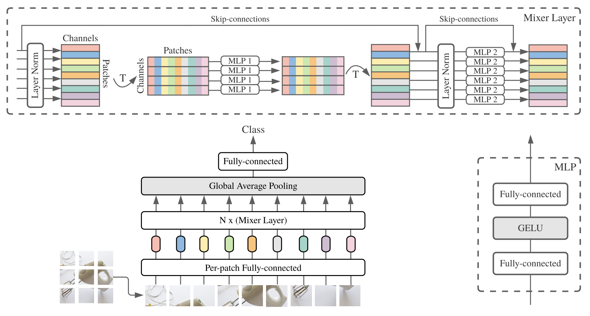
Where:
\[ \begin{array}{ll} \mathbf{U}_{*, i}=\mathbf{X}_{*, i}+\mathbf{W}_2 \sigma\left(\mathbf{W}_1 \operatorname{LayerNorm}(\mathbf{X})_{*, i}\right), & \text{ for } i=1 \ldots C, \text{ (MLP1)} \\ \mathbf{Y}_{j, *}=\mathbf{U}_{j, *}+\mathbf{W}_4 \sigma\left(\mathbf{W}_3 \operatorname{LayerNorm}(\mathbf{U})_{j, *}\right), & \text{ for } j=1 \ldots S. \text{ (MLP2)} \end{array} \]
- \(\mathbf{X} \in \mathbb{R}^{s \times c}\)
- Patches, \(s = 128\)
- Hidden dimension, \(c = 1024\)
- MLP1: \(\mathbf{W}_1 \in \mathbb{R}^{d_s\times s}\), \(\mathbf{W}_2 \in \mathbb{R}^{s\times d_s}\)
- MLP2: \(\mathbf{W}_3 \in \mathbb{R}^{d_c\times c}\), \(\mathbf{W}_4 \in \mathbb{R}^{c\times d_c}\)
- Channel-mixing MLP hidden dimension: \(d_c = 4096\)
- Patch-mixing MLP hidden dimension: \(d_s = 512\)
- Number of Mixer layers: \(24\)
- Batch size: \(1024\)
(a) Calculate the number of FLOPs required to complete a forward and backward pass. You can ignore the embedding layer, pooling, and final fully connected layer. This is a rough calculation, so you can neglect certain operations! You will be marked based on a log scale (be within one order of magnitude of the correct answer). Please show your workings. 10 marks
(b) Calculate the total memory requirements (in MB) for storing all activations during the forward pass of the entire MLP-Mixer model. Assume all values/parameters are stored in 32-bit floating-point format and no gradient checkpointing is applied. Please only consider the activations in the Mixer Layer (you can ignore the embedding layer and global average pooling). 10 marks
(c) Why do the MLP-Mixer authors claim that this architecture has linear complexity with respect to the number of input patches. 1 mark
Question 2: Memory Optimisation Techniques
(a) Explain the concept of gradient accumulation in detail. Specifically, what problem does it solve and how. 6 marks
(b) The following PyTorch code attempts to implement gradient accumulation. Please fill in the required code.
def train_with_gradient_accumulation(
    model, dataloader, criterion, optimizer, accumulation_steps=4
    ):
    model.train()
    optimizer.zero_grad()
    for batch_idx, (data, target) in enumerate(dataloader):
        data, target = data.to(device), target.to(device)
        output = model(data)
        loss = criterion(output, target)

        ###start of code###


        ###end of code###

        if (batch_idx + 1) % accumulation_steps == 0:
            ###start of code###


            ###end of code###
4 marks
(c) Describe gradient checkpointing in detail. How does it trade off computation for memory, and in what circumstances should it be used? 4 marks
Question 3: Mixture of Experts
(a) Briefly describe the Mixture of Experts (MoE) architecture, including its key components and how it differs from standard Transformer models. The following diagram represents a simplified Mixture of Experts layer. As part of your explanation, label each component and explain their functions. Finally detail the motivation behind MoE in the context of scale. 8 marks

(b) Explain the phenomenon of “routing collapse” in Mixture of Experts models, what causes it and detail 2 strategies which can be employed to reduce this issue? 4 marks
Question 4: Parameter-Efficient Fine-Tuning
(a) Consider a pre-trained Transformer block with a hidden dimension of 1024 and 1 attention head. If you apply LoRA with rank \(r=8\) to the query and value projection matrices:
Calculate the number of trainable parameters in the original transformer block projection matrices (k, v, q, o). 3 marks
Calculate the number of trainable parameters with the above LoRA setting. 3 marks
Does LoRA increase or decrease the FLOP count for a forward pass? Explain your answer. 2 marks
(b) The following PyTorch code attempts to implement LoRA for a linear layer. Identify 2 issues with the implementation. Noting that there are 4 issues in total. +2 points for each identified issue and -2 points for incorrect suggestions. Identifying all 4 issues gets you no more marks, just some kudos! The minimum mark for this question is 0.
class LoRALayer(nn.Module):
    def __init__(self, base_layer, rank=4, alpha=1.0):
        super().__init__()
        self.base_layer = base_layer
        self.rank = rank
        self.alpha = alpha

        # Get input and output dimensions from the base layer
        in_features = base_layer.in_features
        out_features = base_layer.out_features

        # Initialise LoRA matrices
        self.lora_A = nn.Parameter(torch.zeros(in_features, rank))
        self.lora_B = nn.Parameter(torch.zeros(rank, out_features))

        # Initialise with random values
        nn.init.normal_(self.lora_A, std=0.02)
        nn.init.normal_(self.lora_B, std=0.02)

    def forward(self, x):
        # Original output
        base_output = self.base_layer(x)


        lora_output = (x @ self.lora_A) @ self.lora_B

        return base_output + lora_output
4 marks
(c) Why for BFloat16 do we need to store a full precision copy of the model weights but in QLoRA we only need one copy of the pretrained weights in NFloat4? 4 marks
(d) LoRA commonly initialises the low-rank matrices such that matrix \(A\) is randomly initialised while matrix \(B\) is initialised to all zeros.
Explain why, despite being initialised to zeros, matrix \(B\) still receives non-zero gradients and is updated during backpropagation. 3 marks
What advantage does this initialisation scheme provide at the start of training? 1 mark
(e) Consider the compute efficiency of LoRA compared to full fine-tuning. For a weight matrix \(W \in \mathbb{R}^{N \times N}\) with LoRA matrices \(A \in \mathbb{R}^{r \times N}\) and \(B \in \mathbb{R}^{N \times r}\) where \(r \ll N\). Derive the total FLOPs for LoRA and show that this approaches \(\frac{2}{3}\) of the full fine-tuning cost when \(r \ll N\). 2 marks