1 Computational Foundations
Modern deep learning is defined by scale. The largest language models contain over a trillion parameters, require terabytes of memory, and demand thousands of petaFLOP compute days to train. Before exploring techniques to make this scale accessible to researchers and engineers with limited resources (you), we must first develop tools for reasoning about the computational requirements of these models.
This chapter develops the fundamental arithmetic of deep learning: how numbers are represented in hardware, how much memory a model consumes during inference and training, and how many floating-point operations each forward and backward pass requires.
1.1 Number Representation
All computation on modern hardware operates on finite representations of numbers. Understanding these representations is essential for reasoning about memory consumption, numerical precision, and the tradeoffs that arise when training at reduced precision.
A bit is a single binary digit taking the value 0 or 1. A byte is a string of 8 bits, capable of representing \(2^8 = 256\) distinct values. In INT8 representation, each number is stored using 8 bits (1 byte). Using a signed representation, INT8 can encode integers in the range \([-127, 127]\), giving \(2^8 = 256\) distinct values.

Integer representations are simple and memory-efficient—each INT8 value occupies exactly one byte—but they cannot represent fractional values or numbers outside a narrow range. We would struggle to do deep learning with this data type. This motivates the use of floating-point systems.
A floating-point number consists of three components (the term “floating point” refers to the fact that the radix point can float relative to the significant digits):
- Sign bit (\(s\)): determines whether the number is positive or negative.
- Exponent (\(e\)): an integer that sets the magnitude (range) of the number.
- Fraction (or mantissa, \(f\)): determines the precision of the number.


When the exponent field is all zeros, the number is called subnormal (or denormalised). Subnormal numbers fill the gap between zero and the smallest normal floating-point value, providing gradual underflow instead of an abrupt jump to zero. However, GPU hardware typically flushes subnormals to zero in reduced-precision formats (FP16, BF16), so the exponent range remains the primary defence against underflow in practice. See Wikipedia: Subnormal number.
The number of exponent bits determines the range (how large or small values can be), while the number of fraction bits determines the precision (how finely values are resolved). Deep learning models are empirically more sensitive to underflow and overflow (range) than to rounding errors (precision). This will be explored in Section 3.3.
Example 1.1 (FP32 Representation) Let’s take a look at the widely used FP32 format, which uses 32 bits (4 bytes) per number. An FP32 number uses 1 sign bit, 8 exponent bits, and 23 fraction bits. The value of a normal FP32 number is given by [1]: \[
\text{value} = (-1)^{\text{sign}} \times 2^{(E-127)} \times \left(1 + \sum_{i=1}^{23} b_{23-i} \, 2^{-i}\right).
\] Consider the bit pattern shown in:  \[
\begin{aligned}
\text{sign} &= b_{31} = 0, \quad (-1)^{\text{sign}} = (-1)^0 = +1 \in \{-1, +1\}, \\[6pt]
E &= (b_{30} b_{29} \dots b_{23})_2 = \sum_{i=0}^{7} b_{23+i} \, 2^{i} = 124 \in \{1, \dots, 254\}, \\[6pt]
2^{(E-127)} &= 2^{124-127} = 2^{-3} \in \{2^{-126}, \dots, 2^{127}\}, \\[6pt]
1.b_{22}b_{21} \dots b_0 &= 1 + \sum_{i=1}^{23} b_{23-i} \, 2^{-i} = 1 + 1 \cdot 2^{-2} = 1.25 \in [1, \; 2 - 2^{-23}), \\[6pt]
\text{value} &= +1 \times 2^{-3} \times 1.25 = \mathbf{0.15625}.
\end{aligned}
\]
\[
\begin{aligned}
\text{sign} &= b_{31} = 0, \quad (-1)^{\text{sign}} = (-1)^0 = +1 \in \{-1, +1\}, \\[6pt]
E &= (b_{30} b_{29} \dots b_{23})_2 = \sum_{i=0}^{7} b_{23+i} \, 2^{i} = 124 \in \{1, \dots, 254\}, \\[6pt]
2^{(E-127)} &= 2^{124-127} = 2^{-3} \in \{2^{-126}, \dots, 2^{127}\}, \\[6pt]
1.b_{22}b_{21} \dots b_0 &= 1 + \sum_{i=1}^{23} b_{23-i} \, 2^{-i} = 1 + 1 \cdot 2^{-2} = 1.25 \in [1, \; 2 - 2^{-23}), \\[6pt]
\text{value} &= +1 \times 2^{-3} \times 1.25 = \mathbf{0.15625}.
\end{aligned}
\]
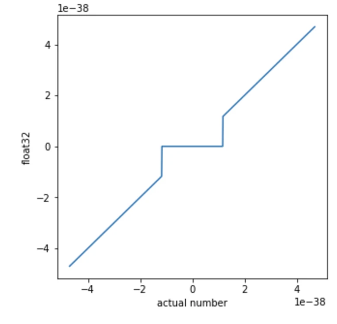
Hidden nonlinearities in “linear” nets (and why ES can exploit them). OpenAI’s Nonlinear computation in deep linear networks [2] highlights a near-zero effect: in float32, very small values can underflow (and with denormals effectively flushed to zero) so the computation has a deadzone / discontinuity around 0. Standard autodiff/backprop differentiates the ideal real-valued ops, so it doesn’t provide a reliable gradient signal to intentionally steer activations into (or exploit) these numerical discontinuities, whereas Evolution Strategies can, because it doesn’t rely on smooth derivatives.
EGGROLL [3] is the complementary tanh-like case: the “activation” comes from the datatype itself, int8 casting and saturated/clipped addition produce a hard-tanh / hard-sigmoid-like saturation at the extremes. Again, this is awkward for vanilla backprop (discrete steps / zero gradients in saturation), but evolutionary optimisation can directly search for parameter settings that benefit from the hardware nonlinearity.
1.2 Memory for Inference
The minimum memory required to run a model at inference time is determined by the number of parameters and the precision at which they are stored.
The memory required to load a model with \(P\) parameters stored at \(B\) bits per parameter is
\[ M_{\text{inference}} = P \times \frac{B}{8} \quad \text{bytes}. \tag{1.1}\]
This formula assumes negligible memory requirements from tokens/represents so batch size 1, a short sequence/context length, and no key–value cache (which we will address in Chapter 4).
Example 1.2 (LLaMA-65B at FP32) For LLaMA-65B [4] stored in FP32: \[ M_{\text{inference}} = 65 \times 10^9 \times \frac{32}{8} = 260 \;\text{GB}. \] This exceeds the memory of any single consumer GPU (an NVIDIA RTX 6000 has 48 GB; an A100 has 80 GB; an H100 has 80 GB). Even in FP16, this model requires 130 GB.
1.3 Memory for Training
Training requires substantially more memory than inference because we must store not only the model parameters but also gradients, optimiser states, and intermediate activations. We build the total memory requirement term by term.
Weights. We still need to load all the model parameters into GPU memory—exactly as at inference time. From Equation 1.1:
\[ M_{\text{weights}} = P \times \frac{B}{8} \quad \text{bytes}. \]
Gradients. For every parameter, we need to store how much it should be adjusted—its gradient with respect to the loss. The gradient tensor has the same shape and precision as the parameter tensor:
During backpropagation, we compute \(\frac{\partial \mathcal{L}}{\partial w}\) for every trainable parameter \(w\). These gradients must all be stored simultaneously because the optimiser updates all parameters together after the backward pass completes.
\[ M_{\text{gradients}} = P \times \frac{B}{8} \quad \text{bytes}. \]
Optimiser states. Knowing the gradient tells us the direction each parameter should move, but not necessarily the best step size. Most optimisers maintain additional per-parameter state to make better update decisions. The Adam optimiser, used in virtually all large-scale training, stores two quantities for every parameter:
Momentum (first moment) smooths the gradient direction across mini-batches, preventing the optimiser from overreacting to any single noisy gradient.
Variance (second moment) tracks the typical scale of each parameter’s gradients, enabling per-parameter adaptive learning rates: parameters in steep directions get smaller steps, parameters in flat directions get larger steps. This prevents the zig-zagging that a single global learning rate would cause in ill-conditioned landscapes.
- First moment (momentum): a running mean of past gradients, \(P \times \frac{B}{8}\) bytes.
- Second moment (variance): a running mean of past squared gradients, \(P \times \frac{B}{8}\) bytes.
\[ M_{\text{optimiser}} = 2 \times P \times \frac{B}{8} \quad \text{bytes}. \]
Putting weights, gradients, and optimiser states together in FP32 (\(B = 32\)):
\[ M_{\text{train}} = \underbrace{4P}_{\text{weights}} + \underbrace{4P}_{\text{gradients}} + \underbrace{8P}_{\text{Adam}} + M_{\text{act}} \quad \text{bytes}, \tag{1.2}\]
where \(M_{\text{act}}\) is the memory consumed by activations—the intermediate values produced during the forward pass that must be retained for backpropagation.
In practice, training is rarely performed entirely in FP32. Mixed-precision training (Section 3.3) uses lower-precision formats (e.g., BF16) for weights, gradients, and activations while maintaining FP32 only for optimiser states, significantly reducing the memory footprint computed above.
Why We Store Activations
Consider a single linear layer that computes \(\mathbf{y} = W\mathbf{x}\) during the forward pass. To update \(W\) via gradient descent, we need its gradient: \[ \frac{\partial \mathcal{L}}{\partial W} = \frac{\partial \mathcal{L}}{\partial \mathbf{y}} \cdot \mathbf{x}^\top. \] This requires \(\mathbf{x}\)—the input to the layer during the forward pass. Similarly, for a nonlinearity such as \(\mathbf{y} = \text{GeLU}(\mathbf{x})\), the backward pass requires \(\mathbf{x}\) to evaluate the derivative \(\text{GeLU}'(\mathbf{x})\).
Many operations in the forward pass must save their input (or output) so that the backward pass can compute correct gradients. For a deep network with many layers, these saved tensors—called activations—accumulate and can consume enormous amounts of memory.
Activation Memory in a Transformer Layer
We now walk through each operation in a single transformer layer [5] and identify the tensors that must be stored for the backward pass. We assume the layer processes a batch of \(b\) sequences of context length \(n\) with hidden dimension \(d\) and \(n_h\) attention heads, and that activations are stored in 4-byte precision (FP32). Dropout masks require only 1 byte per element.
Self-attention sub-layer:
- Layer Norm: stores its input \(\mathbf{X}\) (needed for the normalisation backward pass) \(\to\) \(4bnd\) bytes.
- QKV projection (\(\mathbf{Q}, \mathbf{K}, \mathbf{V} = W_Q \mathbf{X}', W_K \mathbf{X}', W_V \mathbf{X}'\)): stores the layer norm output \(\mathbf{X}'\) (for computing weight gradients) and the projected \(\mathbf{Q}, \mathbf{K}, \mathbf{V}\) (for the attention backward pass) \(\to\) \(4bnd + 3 \times 4bnd = 16bnd\) bytes.
- Attention scores (\(\mathbf{Q}\mathbf{K}^\top / \sqrt{d_k}\)): stores the score matrix before softmax \(\to\) \(4bn_hn^2\) bytes.
- Softmax: stores the output probability matrix \(\to\) \(4bn_hn^2\) bytes.
- Attention dropout: stores the binary mask \(\to\) \(bn_hn^2\) bytes.
- Weighted sum (\(\mathbf{A}\mathbf{V}\)): stores the context vectors \(\to\) \(4bnd\) bytes.
- Output dropout: stores the binary mask \(\to\) \(bnd\) bytes.

Feed-forward sub-layer:
- Layer Norm: stores its input \(\to\) \(4bnd\) bytes.
- First linear (\(d \to 4d\)): stores its input (the layer norm output) \(\to\) \(4bnd\) bytes.
- GeLU activation: stores its input (the \(4d\)-dimensional intermediate) for computing \(\text{GeLU}'\) \(\to\) \(4 \times 4bnd = 16bnd\) bytes.
- Second linear (\(4d \to d\)): stores its input (the GeLU output) \(\to\) \(4 \times 4bnd = 16bnd\) bytes.
- FFN dropout: stores the binary mask \(\to\) \(bnd\) bytes.
Summing these contributions: the ten tensors stored at 4-byte precision contribute \((4{+}16{+}4{+}4{+}4{+}16{+}16) \cdot bnd = 64\,bnd\) bytes, the two dropout masks contribute \(2\,bnd\) bytes, and the attention scores, softmax output, and attention dropout mask contribute \((4{+}4{+}1) \cdot bn_hn^2 = 9\,bn_hn^2\) bytes. For a model with \(L\) layers, the total activation memory is
\[ M_{\text{act}} = L \cdot b \cdot n \cdot \bigl(66d + 9 n_h \cdot n\bigr) \quad \text{bytes}. \tag{1.3}\]
Example 1.3 (LLaMA-65B Training Memory) For LLaMA-65B in FP32 with batch size 1 (note that activations scale linearly with batch size):
\[ \begin{aligned} \text{Weights:} &\quad 4 \times 65 \times 10^9 = 260 \;\text{GB} \\ \text{Gradients:} &\quad 4 \times 65 \times 10^9 = 260 \;\text{GB} \\ \text{Adam states:} &\quad 8 \times 65 \times 10^9 = 520 \;\text{GB} \\ \text{Activations (batch 1):} &\quad \approx 250 \;\text{GB} \\ \hline \text{Total:} &\quad \approx 1{,}290 \;\text{GB} \end{aligned} \]
This would require approximately 25 NVIDIA RTX 6000 GPUs (each with 48 GB), and this is for a batch size of just one….
Do not despair! There are lots of optimisation techniques which can help with this. E.g. you maybe asking why not store the dropout activation masks at 1 bit per element instead of 8 bits? Well, the rest of this series will explore techniques you can use to dramatically reduce this memory footprint.
1.4 FLOPs and Computational Complexity
Beyond memory, we need to quantify the computational cost of running a model. We measure this in floating-point operations (FLOPs). A FLOP is a single arithmetic operation (addition, subtraction, multiplication, or division) on floating-point numbers. We use FLOPs (plural) to denote a count of such operations for a given computation.
The dot product of two vectors \(\mathbf{a}, \mathbf{b} \in \R^n\) requires \[ \FLOPs(\mathbf{a} \cdot \mathbf{b}) = 2n, \] consisting of \(n\) multiplications and \(n-1 \approx n\) additions.
Multiplying an \(n \times p\) matrix by a \(p \times m\) matrix requires
\[ \FLOPs(\mathbf{A} \cdot \mathbf{B}) = 2npm. \tag{1.4}\]
Each of the \(nm\) entries in the output requires a dot product of length \(p\), costing \(2p\) FLOPs.
We now derive the FLOPs for one forward pass through a single transformer layer processing \(n\) tokens with hidden dimension \(d\) and \(n_h\) attention heads (\(d_k = d / n_h\) per head). We use Equation 1.4 throughout.
Self-attention sub-layer:
- Layer Norm: computing the mean, variance, normalisation, scale, and shift involves several element-wise passes over the \(n \times d\) input \(\to \sim 20nd\) FLOPs.
Layer norm and other element-wise operations (GeLU, residual additions) contribute \(O(nd)\) FLOPs, which is negligible compared to the \(O(nd^2)\) and \(O(n^2d)\) terms from matrix multiplications. We include it here in the first instance but drop them from future calculations.
- QKV projections (\(\mathbf{Q}, \mathbf{K}, \mathbf{V} = \mathbf{X}W_Q, \mathbf{X}W_K, \mathbf{X}W_V\)): three matrix multiplications of \((n \times d) \times (d \times d)\) \(\to 3 \times 2nd^2 = 6nd^2\) FLOPs.
- Attention scores (\(\mathbf{Q}\mathbf{K}^\top / \sqrt{d_k}\)): per head, \((n \times d_k) \times (d_k \times n)\); across \(n_h\) heads \(\to n_h \times 2n^2 d_k = 2n^2 d\) FLOPs (since \(n_h d_k = d\)). The scaling by \(1/\sqrt{d_k}\) adds \(n_h n^2\) element-wise operations (negligible).
- Softmax: applied to each row of the \(n \times n\) score matrix for each head. Each row requires \(n\) exponentiations, \(n\) additions, and \(n\) divisions \(\to 3n_h n^2\) FLOPs (negligible).
- Attention \(\times\) Values (\(\mathbf{A}\mathbf{V}\)): per head, \((n \times n) \times (n \times d_k)\); across \(n_h\) heads \(\to n_h \times 2n^2 d_k = 2n^2 d\) FLOPs.
- Output projection (\(W_O\)): \((n \times d) \times (d \times d)\) \(\to 2nd^2\) FLOPs.

Feed-forward sub-layer:
- First linear (\(d \to 4d\)): \((n \times d) \times (d \times 4d)\) \(\to 2n \cdot d \cdot 4d = 8nd^2\) FLOPs.
- GeLU activation: element-wise over \(n \times 4d\) elements (negligible).
- Second linear (\(4d \to d\)): \((n \times 4d) \times (4d \times d)\) \(\to 2n \cdot 4d \cdot d = 8nd^2\) FLOPs.
Summing the dominant terms:
- Self-attention: \(6nd^2 + 2n^2d + 2n^2d + 2nd^2 = 8nd^2 + 4n^2d\)
- Feed-forward: \(8nd^2 + 8nd^2 = 16nd^2\)
- Per-layer total: \(24nd^2 + 4n^2d\)
For an \(L\)-layer transformer with batch size \(B\):
\[ \FLOPs_{\text{forward}} \approx B \cdot L \cdot \bigl(24nd^2 + 4n^2 d\bigr). \tag{1.5}\]
The backward pass requires approximately twice the FLOPs of the forward pass, since we must compute gradients with respect to both the inputs and the parameters at each layer. Thus the total FLOPs for one training step (forward + backward) is roughly \(3 \times\) the forward pass.
Consider a single linear layer \(\mathbf{Y} = \mathbf{X}\mathbf{W}\). The forward pass is one matrix multiplication. The backward pass must apply the chain rule twice: once to compute gradients for the previous layer (\(\frac{\partial \mathcal{L}}{\partial \mathbf{Y}}\,\mathbf{W}^{\!\top}\)) and once to compute gradients for the weights (\(\mathbf{X}^{\!\top} \frac{\partial \mathcal{L}}{\partial \mathbf{Y}}\))—two matrix multiplications.

For a model with \(P\) parameters trained on \(D\) tokens, the total training compute is approximately [6]
\[ \approx 6PD \quad \FLOPs. \tag{1.6}\]
The factor of 6 arises from \(2PD\) for the forward pass, approximately \(2P\) FLOPs per token (each token sees one addition and one multiplication per parameter), summed over \(D\) tokens and \(4PD\) for the backward pass (twice the forward).
Example 1.4 (LLaMA-65B Forward Pass) For LLaMA-65B [7] with model dimension \(d = 8192\), sequence length \(n = 2048\), batch size \(B = 1\), \(L = 80\) layers, and \(n_h = 64\) attention heads, we apply Equation 1.5: \[ \begin{aligned} \FLOPs_{\text{forward}} &= B \cdot L \cdot \bigl(24nd^2 + 4n^2 d\bigr) \\ &= 80 \times \bigl(\underbrace{3.30 \times 10^{12}}_{\text{linear layers}} + \underbrace{1.37 \times 10^{11}}_{\text{attention scores}}\bigr) \\ &= 80 \times 3.44 \times 10^{12} \\ &\approx 2.75 \times 10^{14}. \end{aligned} \] Note that the linear projection terms (\(24nd^2\)) dominate, accounting for \({\sim}96\%\) of the total FLOPs. The quadratic attention terms (\(4n^2d\)) become significant only at much longer sequence lengths.
1.5 Further Reading
- Transformer Inference Arithmetic — a nice breakdown of FLOPs vs Memory Bandwidth bottlenecks.
- JAX Scaling Book — a nice resource for scaling models on TPUs.